Category: Blog

Agentic AI turns your finance stack into a set of closed-loop workflows that plan, execute, and verify analysis—then hand decisions to humans with evidence. Instead of “copilots” that draft text, these agents query governed data, reconcile results, forecast with uncertainty bands, propose actions, and write back to your ARR Snowball, cash, and board packs—under tight controls.

What “agentic” means in finance

Agentic AI is software that can plan, act, and self-check toward a goal—not just chat. It orchestrates a closed-loop workflow (plan → retrieve → act → verify → handoff), running queries and models on governed data, reconciling results, and proposing or executing actions under constraints with audit trails and approvals. In short: an analyst that does the work, not just drafts it. Here are the high level steps that an agentic AI workflow would take:

1. Plans the task (e.g., “explain NRR variance vs. plan”),
2. Retrieves the right definitions and historical context,
3. Acts by running SQL/Python on governed data and using approved tools (forecast libs, optimizers),
4. Self-checks results (unit tests, reasonableness checks),
5. Outputs analysis + recommendations to the target system (Power BI/Tableau, tickets),
6. Asks approval when money or policy is involved.

Think of an analyst who never forgets the metric glossary, never skips reconciliation, and always attaches their SQL.

Where agentic AI adds real leverage

Here are sample agentic AI workflows—grounded in the ARR Snowball and Finance Hub patterns from this blog series—that deliver real leverage. Each use case plans the task, pulls governed data, runs forecasts/causal/optimization models, self-checks results, and writes back actionable recommendations with owners, confidence, and audit trails. Treat these as templates to pilot on top of your existing Fabric/Snowflake/Power BI stack.

1) Close Acceleration & GL Integrity

This use case runs on top of a governed Finance Hub—the daily, finance-grade pipelines outlined in our Resilient Data Pipelines for Finance. With GL, subledgers (AR/AP), billing, bank feeds, payroll, and fixed assets unified with lineage and controls, an agent can pre-close reconcile, flag mispostings and duplicate entries, propose reclasses with evidence, and attach audit-ready notes—shrinking time-to-close while raising confidence in reported numbers.

• Agent: Reconciliation & Anomaly Agent
• Does: auto-matches subledgers to GL, flags mispostings, proposes reclasses with evidence and confidence.
• Tech: embeddings for fuzzy matching, rules + isolation forests, templated journal suggestions.
• Output: a ranked reclass queue with impact to P&L, links to underlying entries, and audit notes.

2) ARR Snowball → Probabilistic Forecast + Prescriptive Actions

Built on the Snowball data model and definitions from ARR Snowball: Proving Revenue Durability, this workflow ingests pipeline, renewals, usage, and billing signals to produce a calibrated forward ARR curve (base/upside/downside bands). It then runs constrained optimization to select the highest-ROI save/expand plays (owners, costs, expected lift) that maximize NRR under budget and capacity, with guardrails and audit-ready lineage.

• Agent: ARR Planner
• Does: converts pipeline/renewals/usage into a probabilistic forward ARR curve; recommends the portfolio of save/expand actions that maximizes NRR under budget/capacity.
• Tech: hierarchical time-series + renewal/expansion propensity; mixed-integer optimization for action selection.
• Output: Base/Upside/Downside bands, top drivers of variance, and a monthly action schedule (owners, due dates).

3) Cash Flow with Contract Awareness

Building on the Cash-Flow Snowball outlined in Extending Snowball to Cash & Inventory, this agent (“Cash Orchestrator”) turns contracts into cash signals: it extracts renewal and payment terms, unifies AR/AP with governed ledger data, and constructs a calendarized view of expected inflows/outflows. From there, it runs a 13-week stochastic cash simulation and proposes term mixes (early-pay incentives, cadence, invoicing options) that improve cash conversion cycle (CCC) without eroding NRR—backed by bi-objective optimization (NPV vs. CCC) and full audit trails.

• Agent: Cash Orchestrator
• Does: extracts terms from contracts, joins AR/AP, simulates collections & payment runs, and proposes term mixes (early-pay incentives, cadence) that improve CCC without hurting NRR.
• Tech: LLM extraction (renewals, uplifts), stochastic cash simulation, bi-objective optimization (NPV vs. CCC).

4) Cost Allocation When Detail Is Thin

Extending the approach in Cost Allocation When You Don’t Have Invoice-Level Detail, this workflow ingests GL lines, vendor metadata, PO text, and operational drivers (products, jobs, regions). An agent uses embeddings and probabilistic matching—constrained to reconcile totals back to the GL—to propose allocations with confidence scores, surface exceptions for human approval, and write back auditable adjustments. The result is consistent product/segment margins and board-ready views even when source detail is sparse.

• Agent: Allocator
• Does: maps GL lines to drivers (products, jobs, regions) using embeddings + historical patterns; produces confidence-scored allocations with human approval.
• Tech: weak supervision, constrained optimization to keep totals consistent with the GL.

5) Variance Analysis that’s Actually Causal

Built on the Snowball definitions from ARR Snowball: Proving Revenue Durability, this agent explains “why” by linking changes in NRR/GRR to causal drivers (onboarding TTV, pricing, usage) with sourced metrics and lineage.

• Agent: Root-Cause Analyst
• Does: traces “why” using causal graphs: e.g., NRR −2 pts ← onboarding TTV +9 days in SMB-Q2 cohort ← implementation staffing shortfall.
• Tech: causal discovery + do-calculus; renders a sourced narrative with links to metrics and lineage.

Reference architecture

This high level reference architecture is used to run agentic AI on your existing lakehouse/warehouse without changing metric logic. It separates concerns into a governed data plane (tables, lineage), a knowledge plane (versioned metric contracts + vector store), a compute/tools plane (SQL/Python, forecasters, optimizers), orchestration (events, schedules, retries), and governance/observability (policy engine, approvals, audit, PII).

Irrespective of the underlying framework, the architecture can work through connectors for Microsoft Fabric, Snowflake, or Databricks and the workflow pattern stays the same, with outputs back to BI (Power BI/Tableau).

• Data plane: governed lakehouse/warehouse; metric contracts (GRR/NRR definitions) in a versioned glossary.
• Tooling: SQL/Python execution sandbox; forecasters (Prophet/ARIMA/Bayesian), optimizers (OR-Tools/pyomo), anomaly libs.
• Knowledge: vector store over metric dictionary, SQL lineage, policy docs (for RAG).
• Orchestration: event triggers (month-end, weekly ARR, daily cash), queue, retries, alerts.
• Governance: policy engine (who can do what), audit log of every query/action, PII redaction, secrets vault.
• UX: push to BI (ARR Sankey/forecast bands), create tickets, and draft board commentary with citations.

How it runs: the agent loop

Now that we’ve covered the use cases and architecture, this list shows the runtime lifecycle every agent follows—plan → retrieve → act → verify → propose → approve → learn—so outputs are consistent, governed, and easy to audit across ARR, cash, and close workflows.

1. Plan: build a step list from the request (“Explain NRR miss in Sept”).
2. Retrieve: pull metric definitions + last 12 months context.
3. Act: run parameterized SQL/Python; if a forecast, produce bands + calibration stats (MAPE/WAPE).
4. Verify: unit tests (sums match GL), reasonableness checks (guardrails), anomaly thresholds.
5. Propose: attach SQL + charts + recommended actions, with impact estimates.
6. Approve: route to owner; on approve, write back tags/notes and schedule the action.
7. Learn: compare predicted vs. actual; update models monthly.

Putting it to work: example workflow map

With the loop defined, here’s how it lands in operations: a simple runbook of when each agent fires, the data/tools it uses, the outputs it produces, and the owner/KPIs who keep it honest. Use this as your starting calendar and adjust SLAs and thresholds to your portfolio.

Workflow	Trigger	Tools & data	Primary outputs	Owner	KPIs
NRR Forecast & Action Plan	Monthly Snowball review	Usage, CRM, billing, optimizer	Forecast bands; top 10 save/expand plays	VP CS / RevOps	NRR Δ, WAPE, action adoption
Close Reconciliation	EOM −2 to +3	GL, subledgers, anomaly detector	Reclass proposals, risk heatmap	Controller	Close time, reclass rate, % auto-accepted
Cash Horizon	Weekly	Contracts, AR/AP, scenarios	13-wk cash projection; term mix recs	CFO	CCC, DSO/DPO, forecast error
Cost Allocation Assist	Monthly	GL, drivers, embeddings	Allocation file + confidence	FP&A	% manual effort saved, variance to audited
Variance Root Cause	On miss > threshold	Snowball, staffing, pricing/events	Causal narrative + corrective plays	FP&A / Ops	Time-to-cause, fix adoption

A simple agent spec (YAML)

To make agents portable and auditable, define them in YAML—a compact, declarative contract that captures the agent’s goal, allowed tools/data, ordered steps (the agent loop), validations/approvals, outputs, and schedule. Checked into Git and loaded by your runner, the same spec can move from dev → stage → prod on Fabric/Snowflake/Databricks with no code changes—just configuration—while enforcing policy and producing consistent, testable results.

agent: arr_planner_v1
goal: "Produce next-12-month ARR forecast with actions to maximize NRR under constraints."
inputs:
  data:
    - table: arr_events # new, expansion, contraction, churn
    - table: usage_signals
    - table: renewals
    - table: opportunities
  glossary: metrics_v1_3 # GRR/NRR, inflow/outflow taxonomy
steps:
  - retrieve_definitions
  - build_features: [renewal_prob, expansion_rate, contraction_rate]
  - forecast_hierarchy: horizon=12, bands=[base,upside,downside]
  - optimize_actions:
      objective: maximize_net_arr
      constraints: {cs_hours<=600, discount_floor>=-15%}
  - validate: [gl_bridge_check, sign_checks, backtest_mape<=0.08]
outputs:
  - forecast_series
  - top_actions: [account, play, owner, expected_lift, cost]
  - narrative_with_citations
approvals:
  - threshold: monetary_impact > 50_000
    approver: VP_Customer_Success
logging: full_sql_and_params

Controls & risk management

Because agentic AI touches dollars and board metrics, it has to run inside hard guardrails. This section defines the essentials: human-in-the-loop approvals for any dollar-impacting change, metric contracts (immutable GRR/NRR and inflow/outflow definitions), full lineage & audit logs for every query/model/output, drift & calibration monitors on forecasts and propensities, and strict privacy/PII controls. Treat these as deployment preconditions—what turns smart helpers into accountable systems your CFO and auditors can trust.

• Human-in-the-loop on money: any dollar-impacting change requires approval.
• Metric immutability: lock GRR/NRR/inflow/outflow in a versioned contract; agents must cite the version they used.
• Lineage & auditability: store SQL, parameters, model versions, and checksums with each output.
• Drift & calibration: monitor forecast error (WAPE/MAPE), probability calibration, and retrain schedules.
• Security & privacy: least-privilege credentials, PII redaction at ingest, fenced prompts (no exfiltration).

Anti-patterns to avoid

These are the failure modes that turn agentic AI from “decision engine” into noise. Dodge them up front and your CFO, auditors, and operators will trust the outputs.

• Unfenced LLMs on production data. No metric contracts, no sandbox—answers drift and definitions mutate.
• “Assistant-only” deployments. Agents that never write back, never learn, and never close the loop (no actions, no feedback).
• Global rates for everyone. One churn/expansion rate across cohorts hides risk; segment or cohort is mandatory.
• Unlogged or unapproved actions. No SQL lineage, no approvals for dollar-impacting changes.
• Moving the goalposts. Changing GRR/NRR or inflow/outflow definitions midstream without versioned metric contracts.
• Double counting. Mixing bookings with ARR before go-live; counting pipeline twice in forecast and Snowball.
• Black-box models. No calibration, drift monitoring, or error bounds—pretty charts, unreliable decisions.
• Security shortcuts. PII/secrets in prompts, excessive privileges, no redaction or audit trails.
• Bypassing orchestration. One-off notebooks/demos with no schedules, retries, or SLAs—results aren’t reproducible.

How to know it’s working

Agentic AI should pay for itself in numbers you can audit. This section defines a small, non-negotiable scorecard—measured against a naïve baseline or A/B holdouts—that agents publish automatically after each run: forecast accuracy and calibration, incremental NRR/cash improvements, action adoption and uplift, and close/reconciliation gains. Targets are set up front (e.g., WAPE ≤ 8%, NRR +Δ pts vs. rank-by-risk, CCC −Δ days), with links to lineage so every win (or miss) traces back to data, SQL, and model versions.

• Close: −X days to close; >Y% anomalies caught pre-close.
• Forecast: portfolio WAPE ≤ 6–8%; calibration within ±2 pts.
• ARR: NRR +Δ pts vs. rank-by-risk baseline; save/expand uplift with A/B evidence.
• Cash: CCC −Δ days; hit rate of collections predictions.
• Productivity: % narratives auto-generated with citations and human-approved.

Conclusion

Agentic AI isn’t about prettier dashboards—it’s about decision engines that plan, act, and verify on your governed data. Tied into ARR Snowball, cash, and cost flows—with definitions, controls, and owners—these workflows compound accuracy and speed, month after month, and turn financial analysis into a repeatable operating advantage.

About K3 Group — Data Analytics

At K3 Group, we turn fragmented operational data into finance-grade analytics your leaders can run the business on every day. We build governed Finance Hubs and resilient pipelines (GL, billing, CRM, product usage, support, web) on platforms like Microsoft Fabric, Snowflake, and Databricks, with clear lineage, controls, and daily refresh. Our solutions include ARR Snowball & cohort retention, LTV/CAC & payback modeling, cost allocation when invoice detail is limited, portfolio and exit-readiness packs for PE, and board-ready reporting in Power BI/Tableau. We connect to the systems you already use (ERP/CPQ/billing/CRM) and operationalize a monthly cadence that ties metrics to owners and actions—so insights translate into durable, repeatable growth.

Snowball is a general-purpose flow lens, not just a SaaS metric. The same Sankey-style visualization that clarifies ARR—inflows, outflows, and the net build with velocity/acceleration—translates cleanly to other operating flows. For cash, it traces invoices and receivables through collections alongside payables and disbursements to reveal net cash build, DSO/DPO, slippage, and CCC. For inventory, it maps receipts to on-hand (by age), then to WIP, shipments/returns, and scrap, exposing turns, DIO, and leakage. Use the same monthly cadence—scorecard, flow diagnostics, actions with owners—to turn hidden movement into decisions that protect runway and margin.

Cash-Flow Snowball (AR ⇄ AP ⇄ Cash)

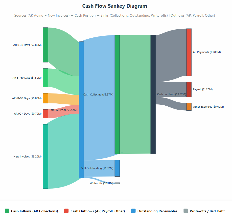
Turning attention to cash flow, the same Snowball lens maps how dollars enter as invoices (AR), age through buckets, and convert to cash—while in parallel showing how purchases become AP and flow out as disbursements. A Sankey-style view makes sources and sinks obvious at a glance (collections, slippage, write-offs; payroll, vendors, taxes), and a monthly scorecard tracks net cash build, its velocity, and acceleration. The result is an operating picture you can act on: tighten or relax payment terms, target early-pay discounts, adjust payment run cadence, prioritize supplier payments, and focus collections where aging migration signals risk. Pair the flow with DSO/DPO/CCC and a simple Collections Efficiency = Cash Collected ÷ (Opening AR + Invoiced) to turn cash visibility into runway and working-capital gains.

What it is. A flow view of dollars from invoices → receivables → cash collected, and from purchases → payables → cash paid, producing a net cash build curve (and its velocity/acceleration) each month. Use a Sankey to show sources (AR aging buckets, new invoices) and sinks (collections, bad debt) alongside outflows (AP aging, payroll, taxes, capex).

Key inputs. AR ledger (invoice dates, due dates, terms, aging), AP ledger (bills, terms), cashbook, payment runs, pipeline-to-invoice assumptions, and expected payment schedules.

Operating metrics & formulas

• Collections Efficiency (period) = Cash Collected ÷ (Opening AR + Invoiced)
• DSO / DPO / CCC: DSO = AR ÷ Avg Daily Revenue, DPO = AP ÷ Avg Daily COGS, CCC = DSO + DIO − DPO
• Slippage: dollars moving from 0–30 → 31–60 → 61–90 → 90+ buckets (leading risk)
• Expected Collections (next 4/8/13 wks) = Σ(Invoice × Probability(bucket, score) × (1 − Dispute%))
• Net Cash Build (velocity) = Ending Cash_t − Ending Cash_{t−1}; Acceleration = ΔVelocity

Operator decisions (examples)

• Tighten terms (shorten from Net45→Net30 where risk is low), early-pay discounts for specific cohorts, or collections playbooks where slippage grows.
• Shift payment runs and renegotiate DPO with low-risk suppliers to compress CCC.
• Prioritize AP by strategic importance (supply-critical vendors first), defer or stage capex.
• Forecast guardrails: hold a minimum cash runway (e.g., ≥ 6× monthly net burn); trigger cost controls if runway breaches.

---

Inventory Snowball (Receipts ⇄ On-Hand ⇄ Consumption/Shipments)

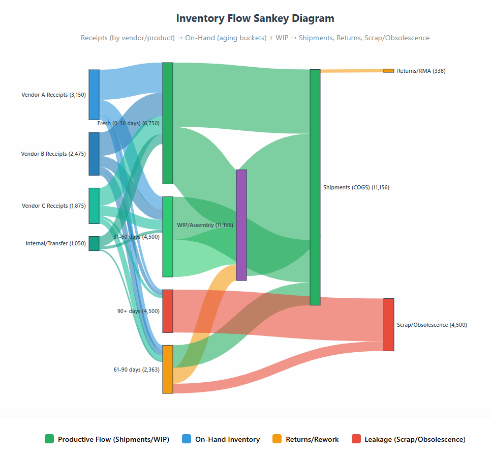
Here’s how the same Snowball lens powers inventory: map receipts into on-hand (by age buckets), through WIP/consumption, and out as shipments/returns/scrap. In a Sankey-style view, link thickness shows volume while color separates productive flow from leakage (shrink, obsolescence). Run it by cohort (receipt vintage), product family, vendor, or location to spot slow movers early, tune ROQ/ROP and safety stock, and align purchasing with real demand. A simple scorecard—net inventory build, throughput velocity, turns/DIO, and leakage—turns visibility into actions like throttling receipts, markdowns, vendor returns, or WIP gating to protect margin and service.

What it is. A flow of units (and dollars) from receipts → on-hand (age buckets) to WIP/consumption → shipments/returns → scrap/obsolescence. Track net inventory build, throughput velocity, and leakage (shrink/obsolete) by cohort (receipt vintage), product family/SKU class, vendor, or location.

Key inputs. Item master, BOM (if applicable), receipts, moves/transfers, WIP, shipments (COGS), returns/RMAs, scrap/obsolescence, forecast, and safety-stock/ROP settings.

Operating metrics & formulas

• Turns = COGS ÷ Avg Inventory; DIO = (Avg Inventory ÷ COGS) × 365
• Aging distribution (0–30/31–60/61–90/90+) by SKU family or vendor
• Obsolescence Rate = Scrap + Write-downs ÷ Avg Inventory
• Fill Rate / OTIF by cohort; Excess Days Supply = On-Hand ÷ Avg Daily Demand
• Inventory Efficiency (period) = Productive Flow (WIP + Shipments) ÷ (WIP + Shipments + Scrap/Obsolescence)

Operator decisions (examples)

• Throttle receipts or replan ROQ/ROP where excess days supply is high; expedite only for cohorts with proven demand velocity.
• Markdown/liquidate aging cohorts before they cross obsolescence thresholds; vendor returns where contracts allow.
• Postponement/late-stage assembly to reduce variant risk; vendor rationalization when shrink/defect rates spike.
• Safety-stock tuning by forecast error and service target; WIP gating if flow is blocked downstream.

Conclusion: one lens for flows that drive value

Extending the Snowball lens to cash and inventory gives you a single way to see—and manage—your most important flows: dollars, units, and revenue. The result is earlier signals and fewer surprises: net cash build with DSO/DPO/CCC guardrails, inventory throughput with turns/DIO and leakage, and the same Sankey-style visibility you use for ARR. Run one monthly cadence—scorecard → flow diagnostics → 2–3 actions with owners—and you’ll turn visibility into working-capital gains, margin protection, and a stronger balance sheet. Lock a simple taxonomy, keep definitions stable, and track movement over time. One lens, three flows: compounding revenue, healthier cash, and smarter inventory—operated to value.

About K3 Group — Data Analytics

At K3 Group, we turn fragmented operational data into finance-grade analytics your leaders can run the business on every day. We build governed Finance Hubs and resilient pipelines (GL, billing, CRM, product usage, support, web) on platforms like Microsoft Fabric, Snowflake, and Databricks, with clear lineage, controls, and daily refresh. Our solutions include ARR Snowball & cohort retention, LTV/CAC & payback modeling, cost allocation when invoice detail is limited, portfolio and exit-readiness packs for PE, and board-ready reporting in Power BI/Tableau. We connect to the systems you already use (ERP/CPQ/billing/CRM) and operationalize a monthly cadence that ties metrics to owners and actions—so insights translate into durable, repeatable growth.

Finance teams live and die by the quality of their numbers. Executives expect reports that are repeatable, auditable, and on time—while operations demand fresh data and engineering just wants systems that don’t break every close. The reality is that finance data isn’t static: source systems update late, postings get rebooked, and every entity has its own timing quirks.

The way through is disciplined data architecture. A resilient pipeline is idempotent (runs twice, lands once), replayable (can reprocess history cleanly), and observable (tells you what ran and what failed). Organize it around a simple, layered pattern—Bronze (raw), Silver (curated), Gold (semantic/reporting)—and enforce clear controls for backfills and late-arriving data.

Get this right and month-end shifts from a scramble to a routine: reproducible for finance, fresh for operators, and calm for engineering.

What We Mean by “Finance Data”

When we talk about finance data, we’re not referring to a single ledger table or dashboard. It’s an ecosystem of structured, governed information that must balance precision with traceability—from monthly summaries all the way down to individual invoices. Finance depends on both the summarized view that closes the books and the granular transactions that explain where every number came from.

Summary-Level Reporting: The Ledger View

At the top of the stack is the governed layer used for financial reporting—your trial balance, chart of accounts, locations, and fiscal calendar. This is where finance teams confirm that debits equal credits, that every account rolls up correctly to a report line, and that each entity is aligned to the proper fiscal period.

The trial balance aggregates balances by account, entity, and period; the chart of accounts defines the financial language—assets, liabilities, revenue, and expense—that underpins every report.
Locations and entities anchor results by site or legal company, and the fiscal calendar dictates how those periods close and roll forward.

Layered on top are standardized sales categories, departments and report lines that map GL accounts into a repeatable P&L structure. These definitions form the backbone of every recurring financial report—the numbers that executives, auditors, and investors expect to match period over period.

Transactional Drill-Downs: The Detail Behind the Numbers

Beneath the summary lies the transactional world that generates those balances. This is where reconciliation, audit trails, and operational insight live. Finance teams need to be able to drill from the GL summary into the individual invoices, journal lines, customers, vendors, and salespeople that created each amount.

On the revenue side, that means access to invoice and order data—customers, items, quantities, prices, discounts, taxes, posting dates, and sales reps—so analysts can trace a line of revenue back to its source. On the expense side, it includes vendor bills, payments, and purchase orders, providing visibility into timing and accruals. Supporting all of this are the customers, vendors, items, and employees that act as shared reference dimensions—the master data that links every transaction to the correct reporting bucket.

Accounts Receivable (AR) and Accounts Payable (AP) use this same data fabric. AR needs consistent customer hierarchies and invoice statuses for aging and collections; AP relies on vendor details, due dates, and payment records for cash planning. Together, these systems form the operational substrate beneath the general ledger—where transactional truth supports financial accuracy.

What “resilience” means for finance data

Once you understand what finance data really encompasses—from the governed trial balance to the line-level invoices that feed it—the next challenge is keeping that ecosystem stable. Finance can’t afford surprises: the same source data should always yield the same result, no matter when or how many times the process runs.

That’s where resilience comes in. In a world of daily extracts, late files, and ever-changing operational systems, a resilient pipeline ensures that finance gets repeatable numbers, operations get freshness, and engineering gets sleep. It’s the difference between firefighting every close and simply rerunning a trusted process.

Resilience centers on three concepts:

• Idempotent. Every step can run twice and land the same result. Use deterministic keys, truncate-and-load or MERGE with natural/surrogate keys, and avoid “append without dedupe.”
• Replayable. Reprocess any window (e.g., “last 45 days”) without one-off scripts. Keep a watermark per source and parameterize transforms by date range.
• Observable. Always answer “what ran, what failed, what changed.” Maintain a run_log (run_id, start/end, rows in/out, status), dq_results (tests, thresholds, pass/fail), and lineage (source files, batch IDs) that finance can see.

For finance, repeatability from the same source is non-negotiable.

Reference architecture blueprint

If resilience is the behavior we want, this is the shape that produces it. The architecture’s job is simple: preserve traceability from raw files to governed outputs, keep history reproducible, and give Finance a single, contracted place to read from. Each layer has a narrow purpose; together they create stable, auditable flow.

• Bronze (raw). Land data exactly as received. Keep file/batch metadata, load timestamps, and source checksums. Store both snapshots (periodic full extracts for sensitive tables like COA) and CDC/deltas (invoices, payments, usage).
• Silver (curated). Normalize types, fix obvious data quality, generate stable surrogate keys, and standardize enums (status codes, currencies). Apply report-line mapping for GL and basic conformance across entities.
• Gold (semantic). Star schemas and a governed semantic model—fact_gl, fact_invoice, dim_customer, dim_item, dim_date, etc.—with measures defined once for BI.

History Without Headaches: SCDs That Reproduce Month-End

You’ve defined the finance data surface (summary + drill-downs) and shaped the pipeline (Bronze/Silver/Gold). The last ingredient is history semantics: how labels, hierarchies, and attributes evolve without breaking prior periods. Month-end trust depends on rerunning any past close and getting the same roll-ups and joins. That’s what slowly changing dimensions (SCDs) provide when they’re applied deliberately—not everywhere, only where the business meaning changes.

• GL Accounts / Report Lines. Usually SCD-1 on names/descriptions (keep current labels), but maintain effective-dated mapping rules so past months reproduce the exact roll-up.
• Customers / Items. Use SCD-2 for attributes that affect analysis (industry, segment, item family). Surrogate keys enable stable joins; valid_from/valid_to makes time-travel simple.
• Reference bridges. For many-to-many (e.g., customer ↔ parent org), use bridge tables with effective dating to keep joins cheap and auditable.

Handling Backfills and Late-Arriving Facts During Close

Even with well-designed SCDs and stable keys, the month-end close is where resilient pipelines prove their worth. This is when new files arrive after cutoff, rebooks shift timing, or manual corrections appear just as finance wants to lock results. Without guardrails, these timing mismatches cause re-runs, mismatched balances, and sleepless nights.

The solution is to design for imperfection—to expect late data, rolling windows, and controlled reprocessing rather than firefighting. A resilient pipeline doesn’t panic when something posts late; it simply replays the window and reconciles automatically.

• Rolling reprocess window. Always recompute the last N days (e.g., 45–60) so rebooks, timing fixes, or late files correct automatically.
• Dual-calendar discipline. Track document date, service period, and posting date. Choose one to drive reporting; persist the others for reconciliation.
• Freeze with exceptions. Let finance “freeze” a period in Gold once signed off; still allow Bronze/Silver updates. Approved adjustments flow via a controlled adjustments table, not ad-hoc edits.
• Deterministic tie-backs. Recompute invoice line totals in Silver and compare to GL in Gold. Variances above a threshold open an investigation item rather than silently passing.

Observability: tests, freshness SLAs, run logs

You’ve designed for history (SCDs) and timing (rolling reprocess with freeze-and-exceptions). The last piece is visibility: when late files or rebooks happen, everyone should immediately see what ran, what’s late, and what changed. Treat data quality like automated QA and expose the operational truth in the same place people read the numbers.

Start with a compact test suite at Silver/Gold—schema/required fields, reconciliations (TB, AR aging, cash), uniqueness on (site, doc_id, line_no), and simple MoM/YoY variance bands. Write every result to a dq_results table with thresholds, owners, and pass/fail, and pair it with a run_log that captures run_id, job, layer, start/end, status, rows in/out, and upstream batch/file identifiers. Then surface both in your BI model so anyone can answer, at a glance, “what’s green, what’s red, and why.”

Publish dataset-level freshness SLAs (e.g., invoices by 06:00; GL by T+1) and show a visible “Data as of …” banner when an SLA is missed. If a site is delayed, don’t block portfolio views—load them, exclude the late site, and label the omission clearly. With these thin contracts (dq_results, run_log, and freshness SLAs) your pipeline behaves like a product: repeatable numbers, transparent delays, targeted fixes—not guessing.

From Pipeline to Trust: Semantic Layer Contracts

After you’ve built resilient Bronze/Silver/Gold flows, the “last mile” is where trust is either confirmed or lost. Treat the Gold layer as a contract, not just a set of tables. That contract defines the public surface area—table names, column names and types, the grain of each table, and the official definitions of measures like Revenue, COGS, and Gross Margin—so they match the finance manual exactly. When the contract is explicit, reports become predictable and auditors stop negotiating definitions.

Stability is the rule. Don’t change columns in place; add new ones, deprecate with a timeline, and maintain a compatibility view so existing dashboards keep working while teams migrate. Keys should be stable (surrogate where needed), names should be durable, and any changes should ship with a clear changelog in the model repo.

Keep the math in one place. Centralize calculations in the semantic layer (DAX or your chosen semantic engine) so every report uses the same measures. If a metric changes, you update it once and every dashboard inherits the fix—no more drift between teams.

Putting It Into Practice

Resilience isn’t a grand theory—it’s a few disciplined habits applied every day. Land Bronze exactly as received (snapshots for small, point-in-time tables; CDC for high-volume facts). Shape Silver for clean types and keys, SCDs where history matters, and effective-dated report-line mappings. Publish Gold as a contract—stable schemas and single-definition measures that mirror the finance manual.

Operationally, reprocess a rolling window so late files and rebooks resolve themselves; freeze closed periods in Gold and route changes through a controlled adjustments lane. Instrument the whole path with run logs, DQ results, and freshness SLAs surfaced in BI so everyone can see what’s green, what’s red, and why.

Do those things consistently and month-end becomes routine: reproducible for finance, fresh for operators, and calm for engineering.

About K3 Group — Data Analytics

At K3 Group, we turn fragmented operational data into finance-grade analytics your leaders can run the business on every day. We build governed Finance Hubs and resilient pipelines (GL, billing, CRM, product usage, support, web) on platforms like Microsoft Fabric, Snowflake, and Databricks, with clear lineage, controls, and daily refresh. Our solutions include ARR Snowball & cohort retention, LTV/CAC & payback modeling, cost allocation when invoice detail is limited, portfolio and exit-readiness packs for PE, and board-ready reporting in Power BI/Tableau. We connect to the systems you already use (ERP/CPQ/billing/CRM) and operationalize a monthly cadence that ties metrics to owners and actions—so insights translate into durable, repeatable growth.

Recurring models, such as SaaS companies, live and die on retention and expansion, not one-time bookings. ARR Snowball decomposes revenue into inflows (new, expansion) and outflows (contraction, churn), yielding clean GRR/NRR and velocity/acceleration trends that expose true revenue durability. Because it’s cohort-aware and definition-consistent, it avoids P&L masking, ties directly to operating levers (pricing, onboarding, CS), and makes forecasts and valuation more defensible—hence its status as the go-to measure of financial soundness in SaaS.

Traditional P&L is great at telling you what happened. ARR Snowball shows how revenue flows—what’s coming in (new logos, expansion) and what’s leaking out (contraction, churn)—so you can see the net build, velocity, and acceleration of growth over time. That makes durability visible, which is exactly what investors pay for.

Why Snowball beats a P&L

A P&L aggregates; Snowball decomposes. By separating inflows and outflows, you expose the levers that actually move valuation:

• Retention and expansion, not just totals. Snowball isolates GRR/NRR, showing whether growth is compounding from the base or masked by constant new-logo replacement.
• Early risk detection. Month-over-month velocity and acceleration reveal when growth is slowing even if the top line still looks fine. Cohorts (by vintage, product, or segment) make where it’s slowing obvious.
• Operational linkage. Because the flows are explicit, you can tie movements to pricing, onboarding, success plays, and renewal hygiene—and measure the effect the very next month.
• Efficiency & LTV. Combine flow with cost-to-serve to monitor LTV, payback, and a simple durability gauge:
  Efficiency = inflow ÷ (inflow + outflow). A rising efficiency trend almost always precedes multiple expansion.

Revenue Flow

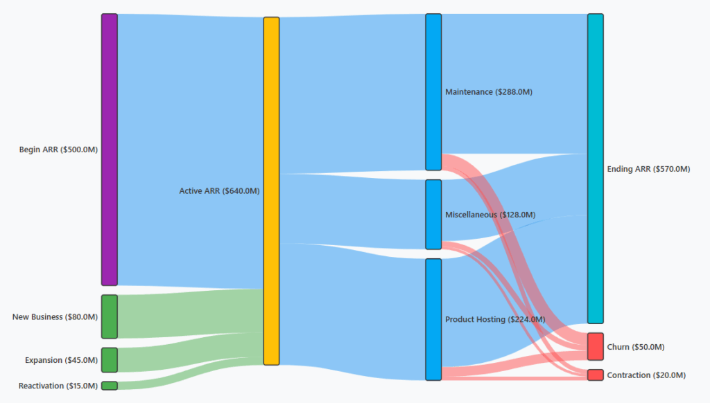
Traditional ARR Snowball analysis focuses on a waterfall chart which shows the net change. A better way to visualize the revenue flow is in a Sankey diagram as outlined below.

A Sankey shows where it came from and where it went—which is what operating and diligence teams need. Using a data cube behind the chart allows deeper analysis by isolating cohorts and breaking down flow through different metrics.

• Provenance → routing → outcome. Starting ARR splits into new, expansion, contraction, and churn streams; link thickness encodes magnitude so leakage is unmistakable.
• One view, many dimensions. You can branch by cohort, product, or segment without creating six separate charts. Colors communicate direction (inflow vs. outflow) instantly.
• Faster pattern finding. Thick outflows from a specific cohort or product highlight where to intervene; thick expansion streams identify “expansion heroes” worth doubling down on.
• Still keep a mini waterfall. A slim row of monthly bars is perfect for net build and velocity; the Sankey carries the richer “how and where” story.

Using this chart as a starting point, an analyst can quickly visualize and drill into problem spots such as churn. Expanding the chart over multiple time periods can show trends and patterns more effectively. The chart also serves as a launchpad for forecasting and planning.

Operating to value

ARR Snowball turns “are we growing?” into “what’s compounding, what’s leaking, and what do we do next?” By visualizing inflows vs. outflows and the net build each month, you get an early-warning system (velocity/acceleration), a shared language with Finance (GRR/NRR), and a single place to assign owners and budget to the highest-yield levers. The outcome is fewer surprises, faster course-corrections, and a consistent story you can defend to the board—and eventually to buyers.

Incorporating the Snowball into monthly planning helps keep management focused on the overall goals instead of their own silos. Here is a monthly agenda that is supported by the accompanying metrics playbook:

• Scorecard: net ARR build, velocity/acceleration, variance to plan.
• Flow diagnostics: top inflow/outflow drivers, cohort hotspots.
• Actions: 2–3 interventions with owners/dates; confirm expected impact.
• Capital allocation: shift dollars/CS capacity where compounding is strongest.

Sample Operating Metrics and Actions

Every organization is different and would have a different mix of metrics to use for monitoring ARR. Here are some common metrics and the resulting actions when the metric is off track:

Metric (formula)	What it signals	Operator decisions & plays
Net ARR Build (Ending ARR − Prior Ending ARR)	Overall compounding pace vs. plan	If down: isolate inflow vs. outflow drivers; assign owners; set 30-day fixes.
Velocity (Δ Net Build MoM) & Acceleration (Δ Velocity MoM)	Early inflection in growth	2+ months negative → review pricing/packaging, onboarding, and save-desk plays; tighten forecast.
GRR ((Base − Outflow on base) ÷ Base)	Renewal hygiene & product-market fit	If < guardrail (e.g., 90–95%): run churn-reason analysis; strengthen 90/60/30 renewal motions; close value gaps.
NRR ((Base − Outflow + Expansion) ÷ Base)	Expansion health & whitespace capture	If flat but GRR OK: launch upsell/cross-sell campaigns; add success plans; adjust bundles/tiers.
Inflow/Outflow Mix & Efficiency (Inflow ÷ (Inflow + Outflow))	Durability of growth	Falling efficiency → prioritize save/expand over net-new; rising → increase growth spend in high-yield segments.
Expansion Mix % (upsell vs. cross-sell)	Which motion drives NRR	Weak cross-sell → enable multi-product plays; rebundle add-ons; revise price fences.
Cohort Health & Hazard (by vintage/product/segment)	Where risk or opportunity concentrates	Red cohorts → assign owner + play (onboarding overhaul, success plan, price/term reset); track monthly impact.
Onboarding Health (time-to-value, activation %)	Predictor of future churn	If TTV slips/activation low → add implementation hours; simplify first-value path; pause deep discounts.
Usage Leading Indicators (seats, feature adoption, logins)	Renewal intent proxy	Dips inside the 90-day window → trigger CS outreach, in-app nudges, exec sponsor calls.
Renewal Ladder (30/60/90 pipeline)	Capacity & focus for CS/deal-desk	Allocate senior reps to high-ARR/at-risk logos; pre-approve save offers; escalate blockers early.
Pricing & Discount Leakage (seen as contraction)	Margin & positioning problems	Tighten discount bands; adjust price fences; rebundle to defend ACV.
Concentration Risk (Top-10 % of ARR)	Resilience & diligence risk	If rising → diversify pipeline; accelerate expansion in under-penetrated segments; scenario-test downside.
LTV & Payback (with cost-to-serve)	Where to invest next	Fund segments with superior LTV:CAC and fast payback; sunset low-yield motions; revisit support model.

Incorporating forecast into the flow

The previous breakdown focused on a historical view, but the same process can be used for future planning and forecasting. The ARR Snowball visualizes your pipeline, renewals, and expansion opportunities into an ARR-based sales forecast: each deal is mapped to a go-live month and ramp, renewals carry probability and expected expansion/contraction, and the result is a forward ARR curve that Sales uses to set targets and coverage, plan capacity/territories, and make in-quarter course corrections. It keeps bookings honest (no double counting before go-live) and turns the forecast into an operating tool—updated monthly as usage and deal health change. Again, different companies would have different metrics to track, but here are a few that could be used:

• Renewal ladder: 30/60/90/180-day schedule with logo/ARR, term, and owner.
• Health & probability: assign a renewal probability by segment/cohort using leading indicators (usage, activation, support load, executive sponsor, discount level).
• Expansion/contraction baselines: segment-level rates (e.g., +x% upsell, −y% contraction) back-tested on the last 12–24 months.
• New business feed: stage-weighted pipeline → ARR start date and ramp curve (e.g., 50% of ACV recognized in month 1, then full run-rate).
• Pricing & terms: planned changes (uplifts, bundles, annual vs. monthly) applied to the right cohorts to prevent double counting.

Conclusion: durable, repeatable growth you can prove

ARR Snowball turns the data you already have into a living operating view—showing where revenue is compounding, where it’s leaking, and what to do next. By separating inflows and outflows and tracking velocity, acceleration, GRR/NRR, and cohort health, you move from retrospective reporting to a monthly cadence of targeted action that compounds value over the hold period.

What you gain, consistently:

• Clarity on revenue quality. A clean record of GRR/NRR, inflow/outflow mix, and cohort durability—so you’re managing compounding ARR, not masking churn.
• A forecast you can run. Renewal ladders, probability-weighted expansions/contractions, and simple scenarios produce a forward ARR curve Sales and Finance both trust.
• Attribution and repeatability. Before/after evidence ties pricing, onboarding, and CS plays to retention and expansion, making wins repeatable.
• Risk transparency. Concentration, contraction pockets, and churn lineage are quantified—with mitigations owned and in motion.
• Valuation logic. Stronger NRR bands, stable cohorts, and steady net build create a defensible bridge from operating metrics to premium multiples.

Bottom line: Snowball gives you truth about the past and signal for the future—then turns that signal into accountable next steps. Use it as your monthly heartbeat to operate to value and keep the revenue story you’ll tell at exit writing itself.

About K3 Group — Data Analytics

At K3 Group, we turn fragmented operational data into finance-grade analytics your leaders can run the business on every day. We build governed Finance Hubs and resilient pipelines (GL, billing, CRM, product usage, support, web) on platforms like Microsoft Fabric, Snowflake, and Databricks, with clear lineage, controls, and daily refresh. Our solutions include ARR Snowball & cohort retention, LTV/CAC & payback modeling, cost allocation when invoice detail is limited, portfolio and exit-readiness packs for PE, and board-ready reporting in Power BI/Tableau. We connect to the systems you already use (ERP/CPQ/billing/CRM) and operationalize a monthly cadence that ties metrics to owners and actions—so insights translate into durable, repeatable growth.

When a company lacks job-level costing, margin analysis stalls. At one client, direct materials, outside services, and labor weren’t tied to jobs; freight revenue was visible, but final freight costs were negotiated monthly with brokers, so the actuals arrived late. We implemented a cost allocation model that provided a transparent, finance-grade allocation for estimating costs at the invoice line level, reconciled to the GL, and scaled across locations.

Why this problem is hard

Solving this problem was not simple. The team was under stressful time pressure because of an event and while the approach was solid, there were nuances that required tweaks due to the realities of the data. The issues below were some complicating factors:

• No job detail: Materials and services hit the GL in aggregate as the movement per month.
• Mixed taxonomies: Sales categories (how revenue is grouped) didn’t align neatly with cost categories (how expenses post).
• Late freight actuals: Costs are re-priced at month-end based on volume discounts, so early views are incomplete.
• Journal entries on GL: Invoice totals didn’t always match GL revenue because of journal entries and other accounting quirks.
• Location nuances: Each location had individual nuances in their accounting such as how sales, costs or freight was tracked.
• Intercompany transfers: Intercompany transfers were handled differently and needed to be removed for calculations.

The goal wasn’t perfection—it was decision-grade estimates that reconcile to the books and hold up in reviews. The algorithm did not account for customer specifics or labor cost which is another important component for margin calculations.

Inputs and setup

The algorithm ran monthly after month-end-close when the books were finalized. Prior to month end, many invoices were still pending, general ledger needed tweaks, and freight cost wasn’t finalized and the algorithm was dependent on each of these sets of monthly data:

• Revenue by sales category from the GL.
• Cost by cost category from the GL.
• Invoice revenue by sales category from invoices.
• Freight cost and revenue from the GL.
• Freight cost and revenue from invoices (some locations tracked cost and others revenue per invoice).
• Weight matrix (management-estimated, per location, per month) indicating how much each cost category contributes to each sales category (weights per cost category sum to 1.0).

Governance: weights are effective-dated, approved by location leadership, and versioned.

Step by step explanation of cost calculation

We start from what’s authoritative—the general ledger. Each month (and for each location), we take the GL cost pools (e.g., Direct Materials, Outside Services) and apportion them to sales categories (e.g., Product, Services, Project, Freight) using a simple, auditable rule: management supplies weights that describe how much each cost category supports each sales category. To make those weights reflect the books, we align invoice revenue to GL revenue once per category. Then we push the allocated dollars down to individual invoices in proportion to line revenue (excluding intercompany), so every invoice line carries a defensible share of costs. Finally, we reconcile back to the GL so totals match and any variance is explained.

Summary of the allocation flow

1. Build the invoice view. For each month and location, sum invoice revenue by sales category, explicitly excluding intercompany lines. This gives the proportional “shape” we’ll use later.
2. Anchor to the ledger. Sum GL revenue by those same sales categories and compute a category-specific scaling factor (GL ÷ invoice). This aligns invoice activity to booked revenue without double-counting.
3. Identify the cost pools. Sum GL cost by cost category (e.g., Direct Materials, Outside Services, Freight Cost). These are the dollar totals you must preserve.
4. Apply management weights. Use the approved weight matrix (cost category × sales category) to blend business judgment with GL-aligned revenue, producing a fair share of each cost pool for each sales category.
5. Turn shares into dollars. Multiply each share by its GL cost pool to get allocated dollars per sales category. Because you allocate from GL costs, category totals remain exact for the month.
6. Push to invoice lines. Within each sales category, distribute its allocated dollars to invoice lines in proportion to line revenue (again, excluding intercompany from the denominator). Now every line carries cost by category, enabling customer, product, and location margin views.
7. Reconcile and log. Verify that the sum of all line allocations equals the GL cost pools (within rounding). Record pass/fail, any variance reason (e.g., timing, credits, exclusions), and approver, so the process is repeatable and audit-ready.

Intercompany handling: Intercompany transfers are removed from the invoice revenue used for weighting and handled under a separate policy (e.g., zero cost on those lines or an “Intercompany” bucket that’s excluded from profitability views).

Detailed calculation sequence

This method allocates monthly GL costs to invoice lines using a management weight matrix, while preserving GL totals. Intercompany (IC) transfers are excluded from invoice revenue used for weighting and handled separately at the end.

1. Aggregate invoice revenue by sales category (exclude intercompany)

   For each location ℓ and month m, sum invoice line revenue for each sales category s, excluding intercompany lines. This builds the invoice-side view used for proportional allocation within the month.

   \[\displaystyle R_{s,\ell,m} \;=\; \sum_{i \in s} \mathrm{LineRevenue}_{i}\]

   Note: The summation is taken over non-intercompany lines only.

2. Aggregate GL revenue by sales category

   From the ledger, compute monthly revenue totals per sales category. This anchors invoice activity to booked revenue for the period.

   \[\displaystyle G_{s,\ell,m} \;=\; \sum \mathrm{GLRevenue}_{s,\ell,m}\]

3. Compute the GL↔Invoice scaling factor per sales category

   Align invoice revenue to GL revenue once per category with a scaling factor. Handle zero or negative invoice totals with a documented fallback (e.g., default to 1.0, carry forward, or skip allocation for that category).

   \[\displaystyle k_{s,\ell,m} \;=\; \frac{G_{s,\ell,m}}{R_{s,\ell,m}}\]

4. Aggregate GL cost by cost category

   Sum monthly GL costs for each cost category c (e.g., Direct Materials, Outside Services, Freight Cost, Labor/Overhead if in scope). These are the dollar pools you will allocate.

   \[\displaystyle C_{c,\ell,m} \;=\; \sum \mathrm{GLCost}_{c,\ell,m}\]

5. Define and approve the cost allocation weight matrix

   Management provides weights w that express how much a cost category contributes to each sales category (by location and month). For each cost category, weights must be non-negative and sum to 1.0. Version, date, and approve these values.

   \[\displaystyle \sum_{s} w_{c,s,\ell,m} \;=\; 1 \quad \text{for each } c\]

6. Compute weighted revenue by (cost category, sales category)

   Blend business judgment (weights) with scaled invoice revenue. Using k ensures shares reflect GL-level revenue without double-scaling later.

   \[\displaystyle W_{c,s,\ell,m} \;=\; w_{c,s,\ell,m} \;\times\; \big(R_{s,\ell,m} \times k_{s,\ell,m}\big)\]

   Alternative: Use GL revenue directly: \[\displaystyle W_{c,s,\ell,m}=w_{c,s,\ell,m}\times G_{s,\ell,m}\]

7. Total weighted revenue per cost category

   Sum the weighted revenue across sales categories to get the denominator for shares.

   \[\displaystyle W_{c,\cdot,\ell,m} \;=\; \sum_{s} W_{c,s,\ell,m}\]

8. Derive allocation shares from weighted revenue

   The share indicates what fraction of a cost category’s GL dollars should be assigned to each sales category this month.

   \[\displaystyle \mathrm{Share}_{c,s,\ell,m} \;=\; \frac{W_{c,s,\ell,m}}{W_{c,\cdot,\ell,m}}\]

9. Allocate GL cost dollars to sales categories

   Convert shares into dollars by multiplying by the GL cost pool. This preserves GL totals by cost category for the month and location.

   \[\displaystyle \mathrm{AllocCost}_{c\to s,\ell,m} \;=\; \mathrm{Share}_{c,s,\ell,m} \times C_{c,\ell,m}\]

10. Push allocated costs down to invoice lines

    Within each sales category s, allocate its share of each cost category to invoice lines in proportion to line revenue (still excluding intercompany lines from the denominator). Sum across cost categories to get total line cost.

    \[\displaystyle \mathrm{LineShare}_{i} \;=\; \frac{\mathrm{LineRevenue}_{i}}{\sum_{j \in s} \mathrm{LineRevenue}_{j}}\] \[\displaystyle \mathrm{LineCost}_{i,c} \;=\; \mathrm{AllocCost}_{c\to s,\ell,m}\times \mathrm{LineShare}_{i}\] \[\displaystyle \mathrm{LineCost}_{i} \;=\; \sum_{c} \mathrm{LineCost}_{i,c}\]

    Intercompany handling: IC lines are excluded from allocation. You may set their line cost to 0, or place into a separate “Intercompany” bucket that is omitted from customer/product profitability views.

11. Reconcile to GL and record variances

    Verify that line-level allocations sum to GL totals for each cost category and month (within rounding). Capture pass/fail status, variance (if any), and reason codes (e.g., timing, credits, exclusions). This makes the method audit-ready.

    \[\displaystyle \sum_{i} \mathrm{LineCost}_{i,c} \;\approx\; C_{c,\ell,m}\]

Notes & guardrails

• Zero/negative revenue: If \[\displaystyle R_{s,\ell,m}=0\], use a policy fallback (e.g., quantity shares, carry-forward weights, or skip that category).
• Weights governance: Effective-date and approve weights monthly; keep rationale by location.
• Freight & late actuals: If freight costs arrive after month end, use a provisional ratio during the month and true-up when actuals post, allocated proportional to freight revenue.

Freight costs that arrive late

Freight must be handled differently than other costs. In the case of freight, some locations included freight in the invoice, so freight cost per invoice was hidden. In other cases, freight cost was on the invoice, but revenue was not. In the final case, freight revenue was on the invoice but cost was not. A site by site adjustment was created to accommodate the differences.

• Provisional allocation: Calculate a trailing-average of GL Freight Cost : GL Freight Revenue ratio per location to provisionally allocate freight cost to freight revenue lines during the month.
• Month-end true-up: When actuals post, compute the delta and reallocate across that month’s freight lines proportional to freight revenue.
• Location differences: When freight was not on the invoice, use the GL Fright Cost as a ratio to the monthly GL Revenue then apply that to each invoice line item. Alternatively when there was freight revenue or cost on the invoice, apply the appropriate ratio adjustment to each line item.
• Audit: Record adjustments with effective dates and rationale.

Handling direct labor and contract labor costs

In this case, labor was not job-coded consistently but manufacturing labor was tracked through COGs. A similar set of calculations could be used to estimate labor cost per line item as a ratio of the revenue.

Next iteration: customer-level adjustments

Different customers can legitimately cost more (or less) to serve due to negotiated terms, volume discounts, SLAs, or complexity. The next iteration introduces customer adjustments while preserving GL totals:

Data model additions

• customer_adjustment table: (location, month, sales_category, customer_id, factor, rationale, approver, valid_from, valid_to)
  • factor > 0 (e.g., 1.15 = 15% uplift; 0.90 = 10% relief).

Computation

1) Start with baseline line costs from the two-stage method above (sales-category allocations pushed down to invoice lines).

2) Apply the customer factor per line (for invoice line i of customer k and cost category c):

\[\displaystyle \widetilde{\mathrm{Cost}}_{i,c} = \mathrm{LineCost}_{i,c} \times \mathrm{factor}_{k,c,\ell,m}\]

3) Renormalize to preserve GL totals for each (location \ell, month m, cost category c):

\[\displaystyle \alpha_{c} = \frac{\mathrm{GLCost}_{c,\ell,m}}{\sum_{i} \widetilde{\mathrm{Cost}}_{i,c}}\]

4) Set the final line cost after scaling:

\[\displaystyle \mathrm{FinalCost}_{i,c} = \alpha_{c} \times \widetilde{\mathrm{Cost}}_{i,c}\]

This ensures customer-level adjustments reallocate costs across invoices and customers but the sum still equals the GL. If you also need to hit explicit customer targets (e.g., contractually specified cost shares), apply raking / iterative proportional fitting to satisfy both the GL total and customer totals while maintaining proportionality.

Controls

• Cap factors (e.g., 0.5–1.5) to avoid extreme swings.
• Version and approve factors monthly; require a rationale (contract clause, SLA, brokered freight rule, etc.).
• Surface a Customer Adjustment Impact report: baseline vs. adjusted margin deltas by customer/product.

Why this works

Again, this is an estimate and can be used for directional assessments, but is not as accurate as job level tracking. It is a good proxy when you do not have job level tracking and you are intending on putting job level tracking in place. It works because:

• Business-informed mapping (weights and customer factors) that’s transparent and versioned.
• GL-tied and reproducible with logged variances and true-ups.
• Actionable detail at the invoice line level for customer, product, and location profitability—improving as more granular data becomes available.

About K3 Group — Data Analytics

At K3 Group, we turn fragmented operational data into finance-grade analytics your leaders can run the business on every day. We build governed Finance Hubs and resilient pipelines (GL, billing, CRM, product usage, support, web) on platforms like Microsoft Fabric, Snowflake, and Databricks, with clear lineage, controls, and daily refresh. Our solutions include ARR Snowball & cohort retention, LTV/CAC & payback modeling, cost allocation when invoice detail is limited, portfolio and exit-readiness packs for PE, and board-ready reporting in Power BI/Tableau. We connect to the systems you already use (ERP/CPQ/billing/CRM) and operationalize a monthly cadence that ties metrics to owners and actions—so insights translate into durable, repeatable growth.

PE teams need numbers that are consistent across systems, comparable across companies, and traceable to transactions. Two situations come up repeatedly and benefit from the same architectural patterns.

Use case 1: One portco, many systems, one cohesive report

Situation. A mid-market company runs multiple ERPs and adjacent tools including billing, HR, CRM, and eCommerce. Month end close is slow, product/customer/job margin is unclear, and every board request becomes a bespoke spreadsheet that takes time from skilled people to produce and validate.

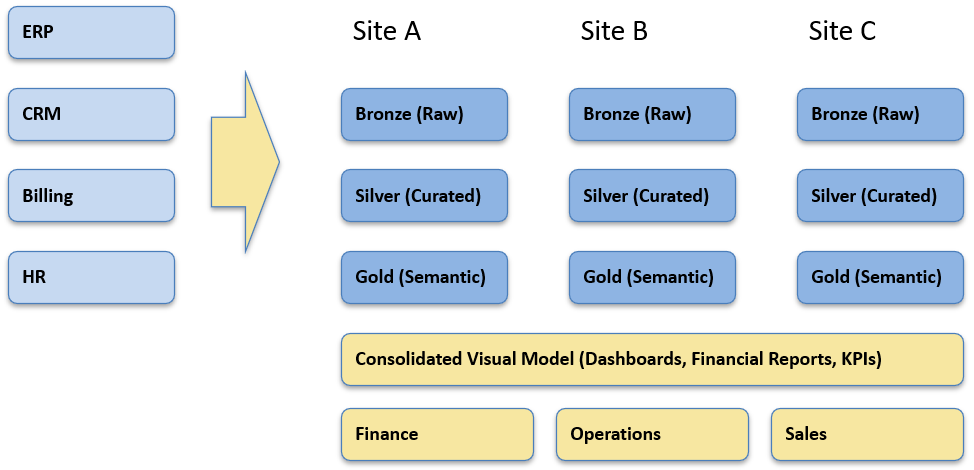
Design choices. Keep each source/location in its own site model (Bronze/Silver) and expose a normalized view in a governed Gold semantic layer. This avoids a brittle, one-time “merge” and lets each dataset evolve independently. GL accounts map to Income Statement/Balance Sheet through an auditable report-line mapping that’s reused in both transforms and rollups. Deterministic, namespaced surrogate keys prevent ID collisions across systems. Reconciliation is part of the product where invoice-level revenue and COGS tie to GL totals, with a variance registry capturing timing and reclass explanations.

What changes for the business. Finance works from IS/BS/Cash that drill to transactions and tie back to the ledger. Unit economics can be examined by product, customer, or job using driver-based allocations with sensitivity checks. Working capital and AR aging are reported consistently across the portco giving insight into cashflow analysis and working capital. Self-service BI through Power BI or Tableau sits on a semantic model that reflects the finance manual, with row-level security and visible “data as of” status.

Use case 2: Portfolio-wide visibility through normalized revenue & cost categories

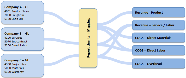
Situation. The sponsor needs a consolidated view across companies with different ERPs and charts of accounts. Today, general ledger reporting categories such as revenue and cost is labeled specifically for that company’s needs and is inconsistent with the other portcos in the portfolio. This limits operators and partners from getting comparable views of company health that quickly diagnose successes or problems.

Design choices. Standardize the definitions, not the systems. We implement an effective-dated report-line mapping that assigns each company’s GL accounts to a common Income Statement structure. Two focal points:

• Sales/Revenue categories. Normalize to a shared set (e.g., Product Revenue, Service/Labor Revenue, Project Revenue, Freight/Handling, Discounts & Rebates, Other Income). Where possible, introduce common Sales Categories as reporting line items in the GL to group operationally similar sales items.
• Cost categories. Normalize COGS into consistent buckets (e.g., Direct Materials, Direct Labor, Subcontract/Outside Services, Freight In/Out, Manufacturing/Shop Overhead, Warranty/Returns) and OpEx into standard lines (e.g., Sales & Marketing, G&A, Operations, Technology). If unit economics are in scope, define allocation rules (e.g., shop overhead to jobs, cloud or distribution costs to products) but keep them versioned and reversible.

Each company retains its own facts/dims and refresh cycle (site models in Bronze/Silver). Portfolio views union those stars in Gold with a Company/Location slicer and a consistent fiscal calendar and FX policy (source, rate type, and timing). Exceptions (e.g., unique revenue treatments, local GAAP nuances) are handled via override mappings with rationale and dates, not ad-hoc edits.

What changes for the business. Sponsors and operators can compare consistent margin and expense structures across entities: revenue by normalized category, gross margin by product/service, COGS composition, and operating expense profiles—drillable to transactions and tied back to GL totals. Board packages, lender updates, and operational reviews draw from the same definitions. One delayed company doesn’t block the view; it’s shown with freshness status and can be temporarily excluded without breaking the portfolio roll-up.

Platform considerations (people and workload first)

Platform selection follows the operating model and who will support it after go-live. We do not dictate technology decisions, rather understand the situation and recommend the best platform for the situcation:

• Microsoft-leaning organizations with minimal IT and Power BI usage. A Fabric-centric stack reduces moving parts: capacity-based compute, OneLake storage, data warehouses and a native semantic model.
• SQL-heavy teams needing strong cost isolation and external sharing. Snowflake provides per-team virtual warehouses and straightforward data sharing.
• Engineering-led teams with notebooks/ML and streaming needs. Databricks (Unity Catalog + Delta) fits open formats and Spark-centric workflows.

Any of these can implement the same pattern—Bronze (raw) → Silver (curated) → Gold (semantic)—with idempotent, replayable pipelines, effective-dated mappings, and visible run logs. The right choice is the one your support staff can confidently operate.

Summary

In both use cases, the value comes from consistent definitions, transaction-level traceability, and an operating model that scales across companies without forcing system uniformity. The patterns above provide a practical checklist when scoping similar work.

About K3 Group — Data Analytics

At K3 Group, we turn fragmented operational data into finance-grade analytics your leaders can run the business on every day. We build governed Finance Hubs and resilient pipelines (GL, billing, CRM, product usage, support, web) on platforms like Microsoft Fabric, Snowflake, and Databricks, with clear lineage, controls, and daily refresh. Our solutions include ARR Snowball & cohort retention, LTV/CAC & payback modeling, cost allocation when invoice detail is limited, portfolio and exit-readiness packs for PE, and board-ready reporting in Power BI/Tableau. We connect to the systems you already use (ERP/CPQ/billing/CRM) and operationalize a monthly cadence that ties metrics to owners and actions—so insights translate into durable, repeatable growth.